Attaching package: 'kableExtra'

The following object is masked from 'package:dplyr':

    group_rows
#Read the penguins_samp1 data file from githubpenguins <-read_csv("https://raw.githubusercontent.com/mcduryea/Intro-to-Bioinformatics/main/data/penguins_samp1.csv")
Rows: 44 Columns: 8
── Column specification ────────────────────────────────────────────────────────
Delimiter: ","
chr (3): species, island, sex
dbl (5): bill_length_mm, bill_depth_mm, flipper_length_mm, body_mass_g, year

ℹ Use `spec()` to retrieve the full column specification for this data.
ℹ Specify the column types or set `show_col_types = FALSE` to quiet this message.
#See the first six rows of the data we've read in to our notebookpenguins %>%head() %>%#if you want a certain number of rows -- add a number in the paranthaseskable() %>%kable_styling(c("striped","hover"))
species
island
bill_length_mm
bill_depth_mm
flipper_length_mm
body_mass_g
sex
year
Gentoo
Biscoe
59.6
17.0
230
6050
male
2007
Gentoo
Biscoe
48.6
16.0
230
5800
male
2008
Gentoo
Biscoe
52.1
17.0
230
5550
male
2009
Gentoo
Biscoe
51.5
16.3
230
5500
male
2009
Gentoo
Biscoe
55.1
16.0
230
5850
male
2009
Gentoo
Biscoe
49.8
15.9
229
5950
male
2009
In the data above we are looking at a data set of penguins. This data set tells us the species of the penguins, which island they are originated from, their bill length and bill depth, flipper length, the mass and sex of each penguin as well as the year they were born.
About our Data
The data we are working with is a data set on Penguins, which includes 8 features measured on 44 penguins. The features included are physiological features (like bill length, bill depth, flipper length, body mass, etc) as well as other features like the year the penguin was observed, the island the penguin was observed on, and the species of the penguin.
Interesting Questions to Ask
Questions I am interested in:
What is the average flipper length of each species?
What species has the penguin with the largest bill length?
What species has the penguin with the largest flipper length?
What is the largest flipper length?
What is the ratio of bill length to bill depth for a penguin? What is the overall average of this metric? Does it change by species, sex, or island?
What is the average body mass? What about by island? By species? By sex?
Are there more male or female penguins? What about per island or species?
Does average body mass change by year?
Data Manipulation
I will be using R code to learn how to manipulate the data, specifically to filter rows, subset columns, group data, and compute summary statistics.
penguins %>%count(island)
# A tibble: 3 × 2
  island        n
  <chr>     <int>
1 Biscoe       36
2 Dream         3
3 Torgersen     5
If we want to filter() and only show certain rows, we can do that too.
#we can filter by sex (categorical variables)penguins %>%filter(species =="Chinstrap")
# A tibble: 2 × 8
species island bill_length_mm bill_depth_mm flipper_le…¹ body_…² sex year
<chr> <chr> <dbl> <dbl> <dbl> <dbl> <chr> <dbl>
1 Chinstrap Dream 55.8 19.8 207 4000 male 2009
2 Chinstrap Dream 46.6 17.8 193 3800 fema… 2007
# … with abbreviated variable names ¹flipper_length_mm, ²body_mass_g
#we can also filter by numerical variablespenguins %>%filter(body_mass_g >=6000) #gives us penguins with a body mass of at least 6000grams
# A tibble: 2 × 8
species island bill_length_mm bill_depth_mm flipper_leng…¹ body_…² sex year
<chr> <chr> <dbl> <dbl> <dbl> <dbl> <chr> <dbl>
1 Gentoo Biscoe 59.6 17 230 6050 male 2007
2 Gentoo Biscoe 49.2 15.2 221 6300 male 2007
# … with abbreviated variable names ¹flipper_length_mm, ²body_mass_g
# A tibble: 7 × 8
species island bill_length_mm bill_depth_mm flipper_l…¹ body_…² sex year
<chr> <chr> <dbl> <dbl> <dbl> <dbl> <chr> <dbl>
1 Gentoo Biscoe 59.6 17 230 6050 male 2007
2 Gentoo Biscoe 49.2 15.2 221 6300 male 2007
3 Adelie Torgersen 40.6 19 199 4000 male 2009
4 Adelie Torgersen 38.8 17.6 191 3275 fema… 2009
5 Adelie Torgersen 41.1 18.6 189 3325 male 2009
6 Adelie Torgersen 38.6 17 188 2900 fema… 2009
7 Adelie Torgersen 36.2 17.2 187 3150 fema… 2009
# … with abbreviated variable names ¹flipper_length_mm, ²body_mass_g
Answering Our Questions
Most of our questions involve summarizing data, and perhaps summarizing over groups. We can summarize data using the summarize() function and group data using group_by().
Let’s find the average flipper length
penguins %>%#average for all speciessummarize(avg_flipper_length =mean(flipper_length_mm))
# A tibble: 1 × 1
  avg_flipper_length
               <dbl>
1               212.
penguins %>%#single species avg lengthfilter(species =="Gentoo") %>%summarize(avg_flipper_length =mean(flipper_length_mm))
# A tibble: 1 × 1
  avg_flipper_length
               <dbl>
1               218.
penguins %>%#average separated by species (grouped average)group_by(species) %>%summarize(avg_flipper_length =mean(flipper_length_mm))
# A tibble: 3 × 2
  species   avg_flipper_length
  <chr>                  <dbl>
1 Adelie                  189.
2 Chinstrap               200
3 Gentoo                  218.
How many of each species do we have?
penguins %>%count(species)
# A tibble: 3 × 2
  species       n
  <chr>     <int>
1 Adelie        9
2 Chinstrap     2
3 Gentoo       33
How many penguins by sex?
penguins %>%count(sex)
# A tibble: 2 × 2
  sex        n
  <chr>  <int>
1 female    20
2 male      24
How many penguins of each species are female? Male?
penguins %>%group_by(species) %>%count(sex)
# A tibble: 6 × 3
# Groups:   species [3]
  species   sex        n
  <chr>     <chr>  <int>
1 Adelie    female     6
2 Adelie    male       3
3 Chinstrap female     1
4 Chinstrap male       1
5 Gentoo    female    13
6 Gentoo    male      20
What is the ratio of bill length to bill depth for a penguin? What is the overall average of this metric? Does it change by species, sex, or island?
We can mutate() to add new columns to our data set.
#average ratio by group penguins%>%group_by(species) %>%mutate(bill_ltd_ratio = bill_length_mm / bill_depth_mm) %>%summarize(mean_bill_ltd_ratio =mean(bill_ltd_ratio),median_bill_ltd_ratio =median(bill_ltd_ratio))
# A tibble: 2 × 3
  island sex     year
  <chr>  <chr>  <dbl>
1 Dream  male    2009
2 Dream  female  2007
Comparing mean bill depth and standard deviation per species.
penguins %>%group_by(species) %>%summarise(mean_bill_depth_mm =mean(bill_depth_mm, na.rm =TRUE),sd_bill_depth_mm =sd(bill_depth_mm, na.rm =TRUE), ) #gives us a mean and sd avearage for each species bill depth
What is the distribution of penguin flipper length?
What is the distribution of penguin species?
Does the distribution of flipper length depend on the species of penguin?
How many penguins were observed per year?
Is there any correlation between the bill length and the bill depth? [scatter plot]\
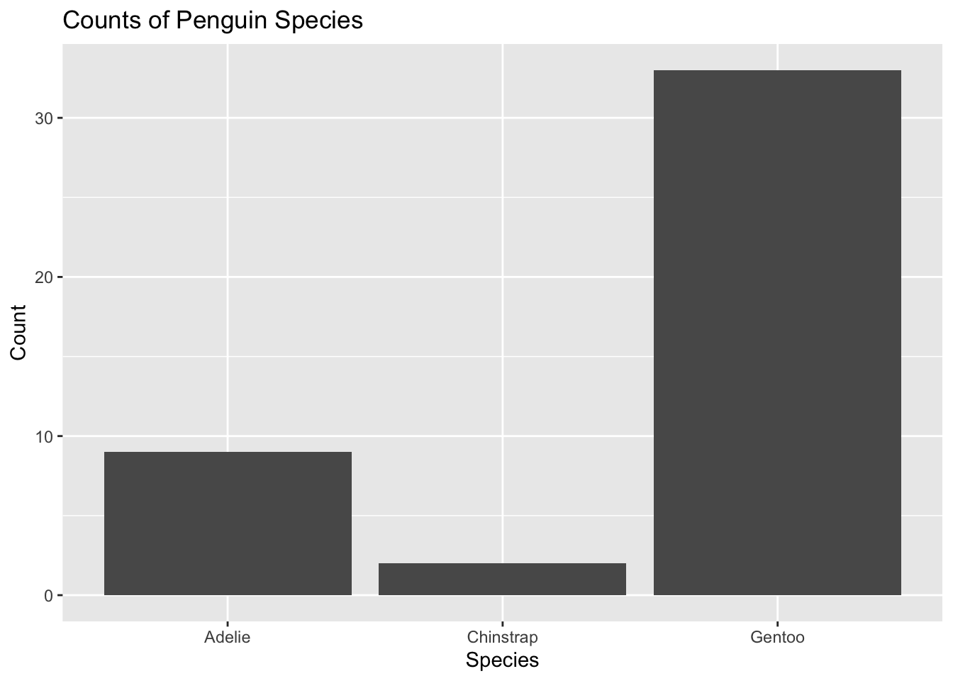
Discussion: In the graph bar plot below we are looking at how many penguins per species were observed.
penguins %>%ggplot() +geom_bar(mapping =aes(x=species))+labs(title ="Counts of Penguin Species",x ="Species", y="Count")
This bar plot depicts the count of each penguins species that were observed. Looking at this diagram we can see that Gentoo’s take over more than 30 of the 44 penguins where as only two Chinstrap penguins were observed. This data tells us that we don’t have an accurate representation of the populations of penguins.
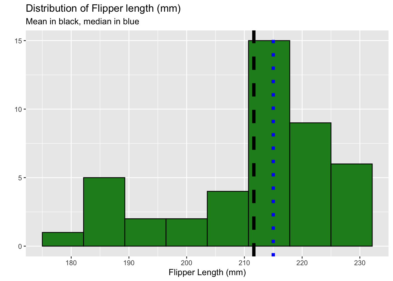
penguins %>%ggplot() +geom_histogram(aes(x=flipper_length_mm),bins =8,fill ="forestgreen",color ="black") +labs(title ="Distribution of Flipper length (mm)", subtitle ="Mean in black, median in blue",x ="Flipper Length (mm)",y ="" ) +geom_vline(aes(xintercept =mean(flipper_length_mm)), lwd =2, lty="dashed") +geom_vline(aes(xintercept =median(flipper_length_mm)), lwd =2, lty="dotted", color ="blue")
Warning: Using `size` aesthetic for lines was deprecated in ggplot2 3.4.0.
ℹ Please use `linewidth` instead.
#more bins = more detail, aes goes back into the data set to find info
This histogram shows the flipper lengths of our data set, outlining the mean (black) and median (blue). We can see that our mean is around 211mm whereas our median is around 215mm. The difference indicates that there may be penguins that were observed who have a relatively small flipper length.
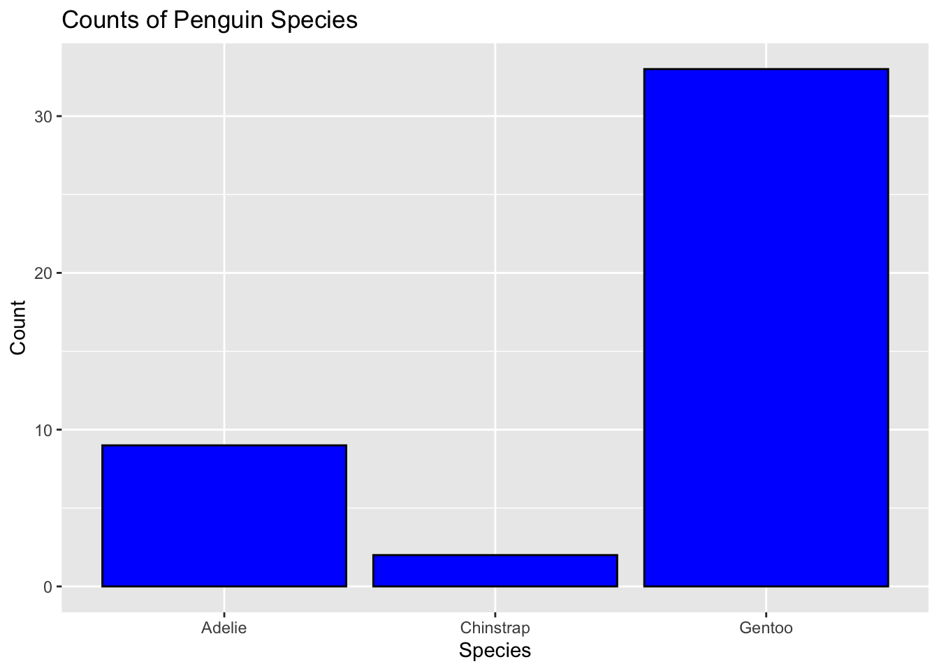
We will now look at the distribution of species.
penguins %>%ggplot()+geom_bar(mapping =aes(x=species), color ="black", fill ="blue") +labs(title ="Counts of Penguin Species",x ="Species", y="Count")
Discussion: This bar plot depicts how many penguins of each species were observed in this dataset. The majority of these penguins are Gentoo’s and we only see 2 Chinstraps that were observed, creating a data set that does not define the whole population of penguins.
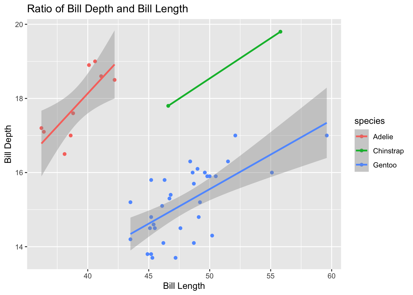
penguins %>%ggplot() +geom_point(aes(x = bill_length_mm, y = bill_depth_mm, color = species)) +labs(title ="Ratio of Bill Depth and Bill Length",x="Bill Length", y ="Bill Depth") +geom_smooth(aes(x = bill_length_mm, y = bill_depth_mm, color = species), method ="lm")
`geom_smooth()` using formula = 'y ~ x'
Warning in qt((1 - level)/2, df): NaNs produced
Warning in max(ids, na.rm = TRUE): no non-missing arguments to max; returning
-Inf
Discussion: This scatter plot answers the question of whether bill length is correlated to bill depth. This diagram shows three different lines, one for each of the species. We can see that the majority of penguins observed are the Gentoo’s which leads us to believe that their line of best fit is more accurate than the other species of penguins that were observed.
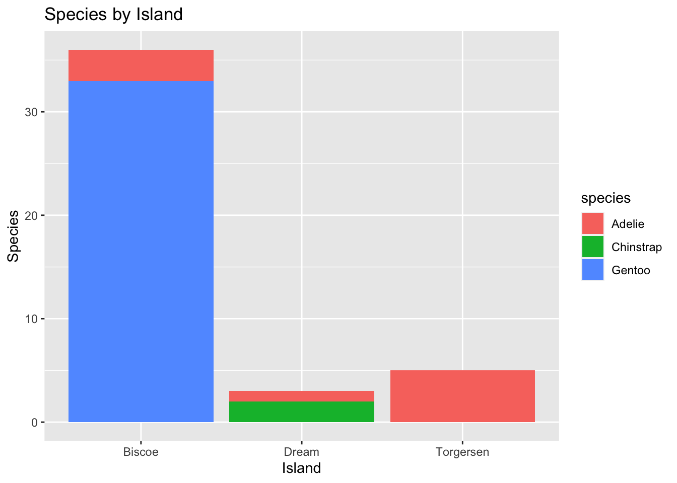
penguins %>%ggplot() +geom_bar(mapping =aes(x = island, fill = species)) +labs(title ="Species by Island",x ="Island",y ="Species")
Discussion: This bar plot depicts how much of each species we observed on each of the three islands. It is noted that all Gentoo’s are found on Biscoe whereas all Chinstraps are found on the island Dream. The species Adelle are found on Biscoe as well as Torgersen.
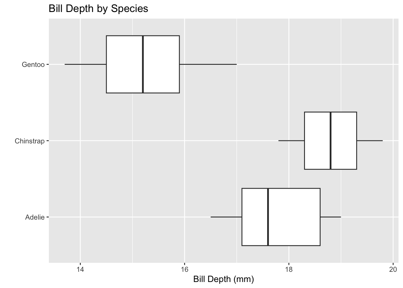
penguins %>%ggplot() +geom_boxplot(mapping =aes(x = bill_depth_mm, y = species)) +labs(title ="Bill Depth by Species",x ="Bill Depth (mm)",y ="")
Discussion: This bar plot explains the bill depth of each species in mm while giving averages for each of the species as well. We can see that Gentoo’s have a smaller average in bill depth where Chinstraps and Adelles are closer to one another.
A Final Question
This chunk of R code tells shows us the confidence interval for mean bill lengths.
    One Sample t-test

data:  penguins$bill_length_mm
t = 1.8438, df = 43, p-value = 0.07211
alternative hypothesis: true mean is not equal to 45
95 percent confidence interval:
 44.87148 47.86943
sample estimates:
mean of x
 46.37045
The average bill length for a penguin that was given from our observations is about 46 mm. This average is defined by only the subset we have observed (44) and cannot be used for the whole population. The data is inaccurate in having only two Chinstrap penguins and a load ful of Gentoo’s, therefore we can say this dataset does not to a good job at portraying the entire population of penguins in the world.